Matlab hold on

The following article provides an outline for Matlab hold on. Matlab’s ‘hold’ command determines whether the newly created graphic object will be added to the existing graph or will it replace the existing objects in our graph. The command ‘hold on’ is used to retain our current plot & its axes properties in order to add subsequent graphic commands to our existing graph.
For example, we can add 2 trigonometric waves, sine and cos, to the same graph using the hold on command.
Hadoop, Data Science, Statistics & others
Syntax:
- Command ‘hold on’ is used to retain the plot in current axes. By doing so, the new plot is added to the existing axes without making any changes to the existing plot.
- Command ‘hold off’ is used to change the hold on state back to off.
Examples of Matlab hold on
Let us see how to add a new plot to the existing axes in Matlab using the ‘hold on’ command.
Example #1
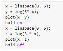
In this example, we will use the ‘hold on’ command to add 2 plots to a single graph. We will plot 2 different logarithmic functions in one graph for our 1 st example.
The steps to be followed for this example are:
- Initialize the 1 st function to be plotted.
- Use the plot method to display the 1 st function.
- Use the ‘hold on’ command to ensure that the plot of the next function is added to this existing graph.
- Initialize the 2 nd function to be plotted.
- Use the plot method to display the 2 nd function.
- Use the ‘hold off’ command to ensure that the next plot, if any, is added as a new graph.
Code:
x = linspace (0, 5);
[Initializing the 1 st logarithmic function]
[Using the plot method to display the figure]
x = linspace (0, 5);
[Initializing the 2 nd logarithmic function]
[Using the plot method to display the figure]
[Using the ‘hold off’ command to ensure that the next plot, if any, is added as a new graph]
This is how our input and output will look like in the Matlab command window.
Input:
Output:
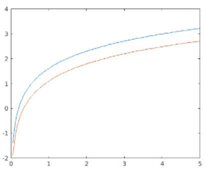
As we can see in the output, we have obtained 2 logarithmic functions in the same graph as expected by us.

Example #2
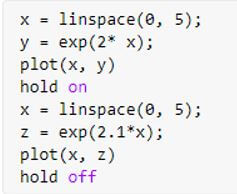
In this example, we will use the ‘hold on’ command to add 2 different exponential functions in one graph.
The steps to be followed for this example are:
- Initialize the 1 st function to be plotted.
- Use the plot method to display the 1 st function.
- Use the ‘hold on’ command to ensure that the plot of the next function is added to this existing graph.
- Initialize the 2 nd function to be plotted.
- Use the plot method to display the 2 nd function.
- Use the ‘hold off’ command to ensure that the next plot, if any, is added as a new graph.
Code:
[Initializing 1st exponential function]
[Using the plot method to display the figure]
[Initializing 2 nd exponential function]
[Using the plot method to display the figure]
[Using the ‘hold off’ command to ensure that the next plot, if any, is added as a new graph]
This is how our input and output will look like in the Matlab command window.
Input:
Output:
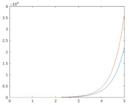
As we can see in the output, we have obtained 2 exponential functions in the same graph as expected by us.
In the above 2 examples, we saw how to add 2 functions to a single graph. We can also use the same ‘hold on’ command to add more than 2 functions also. Next, we will see how to add 3 functions to the same graph.
Example #3
In this example, we will use the ‘hold on’ command to add 3 plots to a single graph. We will plot 3 different exponential functions in one graph for this example.
The steps to be followed for this example are:
- Initialize the 1 st function to be plotted.
- Use the plot method to display the 1 st function.
- Use the ‘hold on’ command to ensure that the next plot is added to this existing graph.
- Initialize the 2 nd function to be plotted.
- Use the plot method to display the 2 nd function.
- Use the ‘hold on’ command to ensure that the next plot is added to this existing graph.
- Initialize the 3 rd function to be plotted.
- Use the plot method to display the 3 rd function.
- Use the ‘hold off’ command to ensure that the next plot, if any, is added as a new graph.
Code:
[Initializing 1st exponential function]
[Using the plot method to display the figure]
[Initializing 2 nd exponential function]
[Using the plot method to display the figure]
[Initializing 3 rd exponential function]
[Using the plot method to display the figure]
[Using the ‘hold off’ command to ensure that the next plot, if any, is added as a new graph]
This is how our input and output will look like in the Matlab command window:
Input:
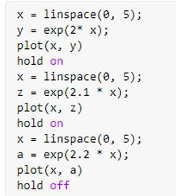
Output:
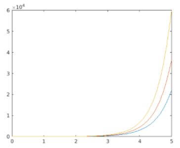
As we can see in the output, we have obtained 3 exponential functions in the same graph as expected by us.
Conclusion
Matlab’s ‘hold on’ command is used to add more than 1 graphic object to the same figure. This command is used to retain our current plot & its axes properties in order to add subsequent graphic commands to our existing graph.
Recommended Articles
This is a guide to Matlab hold on. Here we discuss the introduction to Matlab hold on along with examples for better understanding. You may also have a look at the following articles to learn more –
Построение графиков с двумя независимыми осями в Matlab
Статья будет полезна тем, кто оформляет графики в среде Matlab.
При подготовке графиков для публикации статей в научных журналах и различного рода отчетов, я довольно часто сталкивался с необходимостью построения нескольких кривых, относящихся каждая к своей оси — чтобы не перегружать статью графиками и не выходить за их лимит. Но для этого в Matlab до версии R2014a была лишь команда plotyy(X1,Y1,X2,Y2), которая имеет ряд неприятных особенностей, из-за которых приходилось пользоваться другими программами и делать все вручную, что во-первых, усложняет этот процесс с точки зрения единой стилистики, во-вторых требует большого количества времени, а в-третьих не позволяет оперативно вносить изменения.
К таким неприятным особенностям я бы отнес:
1. Отсутствие аналога hold on («родной» hold on работает не совсем корректно с plotyy). Для того, чтобы добавить более, чем 2 кривые необходимо использовать вот такую конструкцию:
Из этой конструкции вытекает неприятная особенность №2:
2. Размерности массивов, заключенных в квадратные скобки должны совпадать, т.к. из них формируются матрицы элементов. На практике такое бывает очень не часто.
3. Оформление серьезно страдает оттого, что нельзя программными методами изменить цвета и типы всех линий подряд, можно форматировать только набор линий, относящихся к конкретной оси (hLine1 и hLine2) — во всяком случае, я не смог. При этом, я не говорю сейчас об изменении параметров руками, т.е. редактированием в окне «figure» — только непосредственно кодом в .m-файле.
Резюмируя вышесказанное: plotyy() не очень хорошо подходит для отображения нескольких наборов графиков для разных осей. Разве что для простеньких зависимостей типа этих:
То ли дело команда yyaxes, появившаяся в версии Matlab R2014a. Вот тут уж нам стало где развернуться.
Рассказать о прелестях данной команды я бы хотел на своем примере. Задача состоит в том, что мне необходимо построить на одном графике 3 профиля температур (решения, полученные прямым численным методом, моментным методом и экспериментальные значения), относящихся к правой оси, и 3 профиля давлений, относящихся к левой оси. А также добавить стрелки и подписи.
Команды yyaxis left и yyaxis right позволяют справиться с этой задачей на раз. В чем, собственно, суть. В рамках одной figure мы можем построить любое количество графиков, привязав их к одной из осей. В рамках каждой из команд прекрасно работает все то же самое, что и для обычных графиков.
Структура рисунка в таком случае будет выглядеть так:
Наполнив эту структуру необходимым, получаем в результате:
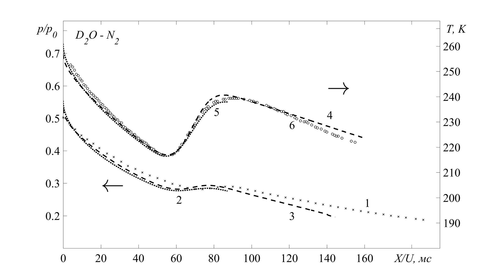
Еще одна дополнительная фишка в подготовке графиков к печати — это их простое и удобное сохранение в любом, поддерживаемом Matlab-ом, формате. Для этого необходимо лишь добавить следующие строки:
Начиная с версии R2014a Matlab стал подходящей программой для подготовки графиков к публикации статей в различных научных журналах. Важным плюсом является очень хорошая гибкость этого инструмента, позволяющая обрабатывать результаты и представлять их в удобоваримом и красивом виде, в том числе и для т.н. «пакетной» обработки.
The Plot Function
The plot function in Matlab is used to create a graphical representation of some data. It is often very easy to «see» a trend in data when plotted, and very difficult when just looking at the raw numbers.
The Plot Function
The plot function usually takes two arguments (but can take one). The first is the X values of the points to plot, and the second is the Y value of the points to plot. Below is an example of creating and plotting the values of the X squared graph from -10 to +10. In the case of a single argument, the X axis becomes 1,2,3,4. up to the length of the array, and the Y axis contains the values of the array.
Notice that plot will «connect the dots» for you, drawing lines between each set of X,Y values.
Single Argument to Plot
If you have a single array that you wish to plot, and don’t really care about the X axis, you just want to see the values plotted in the Y axis, you can pass a single array to the plot function. Here is an example:
Labeling your Plot
The following functions are almost always used with plot to make the output more readable.
- xlabel, ylabel : Provide a labeling for the graph axii.
- title : Provide a title for the graph.
- legend: Provide a legend telling what multiple graph lines mean.
- grid: Put a checkered grid over the graph (add more lines to (sometimes) make it easier to see values.
- axis: Tell how big of an area the graph should display.
The «clf» command
Sometimes you will want to «clear» the figure. This is normally done by simply «plotting» the next thing you want. Alternatively, you can use the «clf» command:
The «hold» command
Sometimes you will want to plot multiple graphs on the XY axis (on the same figure). In Matlab, when you use the plot function more than once, each time you call it, the previous figure is «erased».
To make a previous figure remain on the plot, we use the «hold on;» command. When we want to resume clearing the figure for each new plot, we use the «hold off;» command.
Try the following code:
You should have only seen one graph, the cubed graph (which was the second plot above). Now try this code, using the «hold on;» command.
The «subplot» command
Sometimes you will want to place multiple plots side by side on a single figure. You can achieve this by using the Matlab subplot function.
For many more details on this function (as well as the commands and functions mentioned above) you can always use the help command at the Matlab prompt.
The parameters used by the subplot function determine how many rows and columns for the overall «matrix» of figures, and then which of these positions to put the next plot in. The parameters are: 1) The number of rows, 2) the number of columns, 3) which of the sub plots to use.
Here is an example of how to create a 2×3 matrix (6 figures) of plots and to address each one of them by a number (shown below). Notice how row 1, column 1, is identified by the number 1. Row one, column three is identified by 3. Row two, column one, «wraps» and is identified by 4.:
| Columns | ||||
|---|---|---|---|---|
| one | two | three | ||
| Rows | one | 1 | 2 | 3 |
| two | 4 | 5 | 6 | |
Test this code. Notice that the subplot command stays the same, except for the «index» into which matrix location you want. Also notice that you can title, label, etc, each plot.
Various additional plotting methods
Matlab provides several well known graphing functions, including histograms, pie charts, and stem charts.
Histograms: Histograms are used to show how many values in an array of values fall within certain «bins». For example, if we have the scores of all students on a test, we may want to find out how many scores were between 90-100, 80-90, 70-80, etc. The histogram is the perfect tool for this.
Pie Charts: Pie Charts are useful for showing what percentage of a whole, each element represents. For example, if we knew there were 40 hours in the week, we could use a pie chart to show how many hours were spent on study, sleep, play, etc
Stem Charts: The stem chart draws a line from the bottom of the graph to the appropriate Y value for each X value. For example if the X axis represents how many times a letter was found in a document, we could use a stem plot to show the relationship between all letters, and how often they occur..